本文将对QAT的一些基本算法做一些介绍,然后介绍两种较为直观也较为常用的QAT算法
QAT
首先写出原始形式的量化式:
$$
s \cdot {\rm clamp}(\lfloor \frac{x}{s} \rceil;n,p)
$$
或:
$$
s \cdot [{\rm clamp}(\lfloor \frac{x}{s} \rceil + \lfloor z \rceil;n,p) - \lfloor z \rceil]
$$
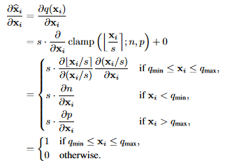
STE(直通估计器)最早在Estimating or Propagating Gradients Through Stochastic Neurons for Conditional Computation中提出。由于round运算的梯度为0或未定义,STE将舍入算子的梯度近似为1:

所以舍入值(权重和激活)相对于原值的导数可以定义为:
LSQ
本文主要提出了两种方法:
- 提供了一种简单的方法来近似量化器步长的梯度,它对量化的状态转换很敏感,可以说在学习步长作为一个模型参数时提供了更精细的优化。
- 提出了一个简单的启发式方法,使步长更新的幅度与权重更新达到更好的平衡,以改善收敛性。
LSQ这一工作引入了可学习的步长$s$:
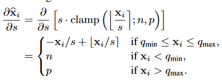
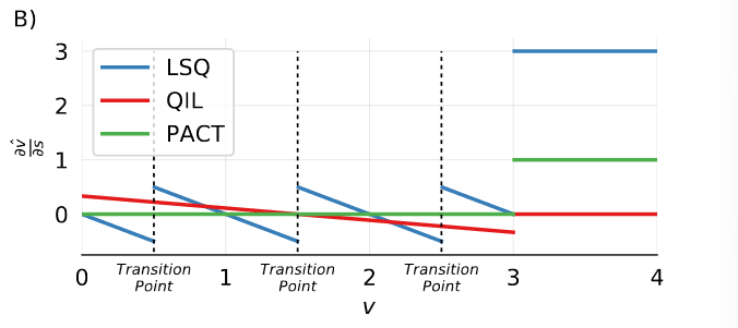
LSQ的巧妙之处在于,它模拟了量化过程中的一个现象:一个给定的$x_i$离量化过渡点越近,它就越有可能由于对$s$的更新改变其量化值$\hat x_i$,导致$\hat x_i$出现大幅度跳跃——梯度随着$x_i$到过渡点的距离减少而增加。
在更新之前,激活和权重的初始步长值为:
$$
s_{init} = \frac{2\bar x}{\sqrt{p}}
$$
在训练过程中,我们期望步长参数随着精度的提高而变小(因为数据被更精细地量化),而步长更新随着量化项目的增加而变大(因为在计算其梯度时,更多的项目被加在一起)。对此我们需要将总损失与一个调节参数相乘:$g=1/\sqrt{n p}$($n$为每一层权重/激活的参数量)。同时将所有矩阵乘法层的输入激活和权重设置为2位、3位、4位或8位,但第一层和最后一层始终使用8位。
LSQ+
LSQ方法大多基于以ReLU为激活函数的模型。但对于GeLU这样的函数,正负范围分布不均,无论是使用无符号量化范围量化(将所有负值钳制为0)还是使用有符号量化范围量化(对激活函数的负和正部分给予同等重视)都会造成精度损失。
LSQ+这一工作引入了可学习的偏置$z$:
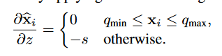
这样,我们就可以在激活处执行非对称量化,提高精度。
对于权重,我们使用对称量化:
$$
s_{init} = \max(|\mu - 3\sigma|,|\mu + 3\sigma|) / 2^{b-1}
$$
对于激活,我们通过校准最小化下式:
$$
s_{init}, \beta_{init} = \arg \min_{s,\beta} ||\hat x - x||_F^2
$$
PACT
本文解决了量化中的一个核心问题:如何在range和precision之间寻找到tradeoff。特别是对于激活来说,这一问题尤其严重。绝大多数activation集中在某个很小的范围,但总有一些outlier点 会离中心非常远。这些outlier的value比较大,如果删除的话,会造成较大的误差。但是,如果你用outlier的最大值来作为range来量化整个数据,又面临着precision不够的问题。
传统的激活函数没有任何可训练的参数,因此量化激活产生的误差无法用BP算法补偿。而传统的ReLU函数输出值域是无界的,这造成了更大的动态范围误差。
PACT函数的定义如下:
$$
y = PACT(x) = 0.5 (|x| - |x-\alpha| + \alpha)
$$
随后是其量化过程:
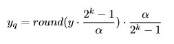
更新$\alpha$的梯度表达式如下(注意到计算第一次倒数时使用了一个直通估计器):
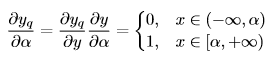
注意到此处的scaling factor并非通过传统方法得到,因此量化表达式有较大的差异。重新改写上式:
$$
s \cdot {\rm clamp}(\lfloor \frac{x}{s} \rceil;0,\alpha), s = \frac{\alpha}{2^k -1}
$$
Code
首先给出PyTorch中自定义求导算子的写法官方文档:
 1
 2
 3
 4
 5
 6
 7
 8
 9
10
11
12
13
14
|
class Exp(Function):
    @staticmethod
    def forward(ctx, i):
        result = i.exp()
        ctx.save_for_backward(result)
        return result

    @staticmethod
    def backward(ctx, grad_output):
        result, = ctx.saved_tensors
        return grad_output * result

# Use it by calling the apply method:
output = Exp.apply(input)
|
借助此,我们可以自定义函数的正向传播和反向传播过程。以下代码参考自。
STE
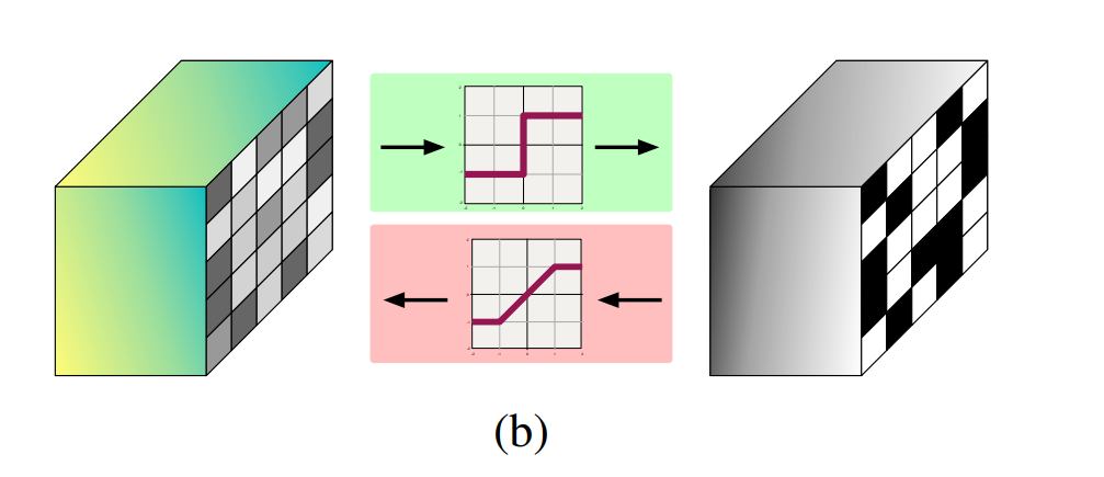
首先我们给出BNN中STE(效果如下图所示)的表达式:
1
2
3
4
5
6
7
8
|
class STEFunction(torch.autograd.Function):
    @staticmethod
    def forward(ctx, input):
        return (input > 0).float()

    @staticmethod
    def backward(ctx, grad_output):
        return F.hardtanh(grad_output)
|
在真正作为一个module使用时,需要进行封装:
1
2
3
4
5
6
7
|
class StraightThroughEstimator(nn.Module):
    def __init__(self):
        super(StraightThroughEstimator, self).__init__()

    def forward(self, x):
        x = STEFunction.apply(x)
        return x
|
对于一般的round函数,其STE可以做如下构造:
1
2
3
4
5
6
7
8
|
class STE(torch.autograd.Function):
    @staticmethod
    def forward(ctx, x):
        return torch.round(x)

    @staticmethod
    def backward(ctx, grad_output):
        return grad_output.clone()
|
我们可以看下这种写法和直接使用torch.round()函数的区别:
 1
 2
 3
 4
 5
 6
 7
 8
 9
10
11
12
13
14
15
|
# original
print('version 1')
x = torch.tensor([0., 100., 200.], requires_grad = True)
out = x.round()
loss = out.mean()
loss.backward()
print(x.grad)

# modified
print('version 2')
x = torch.tensor([0., 100., 200.], requires_grad = True)
out = STE.apply(x)
loss = out.mean()
loss.backward()
print(x.grad)
|
1
2
3
4
|
version 1
tensor([0., 0., 0.])
version 2
tensor([0.3333, 0.3333, 0.3333])
|
可以看到,原生的round函数不产生任何梯度。
此外,还有一种更精妙的写法:
1
2
3
4
|
def round_pass(x):
    y = x.round()
    y_grad = x
    return y.detach() - y_grad.detach() + y_grad
|
此函数的意味是:函数的返回值为y - y_grad + y_grad = x.round(),但反向传播的梯度仍然按照y_grad = x的梯度去算。
按照此种写法还可以实现“梯度倍增”的效果:
1
2
3
4
|
def grad_scale(x, scale):
    y = x
    y_grad = x * scale
    return y.detach() - y_grad.detach() + y_grad
|
LSQ
LSQ的正向传播和反向传播在STE的基础上实现,同时还有初始化规则:
 1
 2
 3
 4
 5
 6
 7
 8
 9
10
11
12
13
14
15
16
17
18
19
20
21
22
23
24
25
26
27
28
29
30
31
32
33
34
35
36
37
38
39
40
41
|
class LsqQuan(Quantizer):
    def __init__(self, bit, all_positive=False, symmetric=False, per_channel=True):
        super().__init__(bit)

        if all_positive:
            assert not symmetric, "Positive quantization cannot be symmetric"
            # unsigned activation is quantized to [0, 2^b-1]
            self.thd_neg = 0
            self.thd_pos = 2 ** bit - 1
        else:
            if symmetric:
                # signed weight/activation is quantized to [-2^(b-1)+1, 2^(b-1)-1]
                self.thd_neg = - 2 ** (bit - 1) + 1
                self.thd_pos = 2 ** (bit - 1) - 1
            else:
                # signed weight/activation is quantized to [-2^(b-1), 2^(b-1)-1]
                self.thd_neg = - 2 ** (bit - 1)
                self.thd_pos = 2 ** (bit - 1) - 1

        self.per_channel = per_channel
        self.s = torch.nn.Parameter(torch.ones(1))

    def init_from(self, x, *args, **kwargs):
        if self.per_channel:
            self.s = torch.nn.Parameter(
                x.detach().abs().mean(dim=list(range(1, x.dim())), keepdim=True) * 2 / (self.thd_pos ** 0.5))
        else:
            self.s = torch.nn.Parameter(x.detach().abs().mean() * 2 / (self.thd_pos ** 0.5))

    def forward(self, x):
        if self.per_channel:
            s_grad_scale = 1.0 / ((self.thd_pos * x.numel()) ** 0.5)
        else:
            s_grad_scale = 1.0 / ((self.thd_pos * x.numel()) ** 0.5)
        s_scale = grad_scale(self.s, s_grad_scale)

        x = x / s_scale
        x = torch.clamp(x, self.thd_neg, self.thd_pos)
        x = round_pass(x)
        x = x * s_scale
        return
|
LSQ+同理,只不过在原有基础上引入偏移量z,并使用不同的初始化规则,此处不再详细说明。
PACT
 1
 2
 3
 4
 5
 6
 7
 8
 9
10
11
12
13
14
15
16
17
18
19
20
21
22
|
class LearnedClippedLinearQuantization(nn.Module):
    def __init__(self, num_bits, init_act_clip_val, dequantize=True, inplace=False):
        super(LearnedClippedLinearQuantization, self).__init__()
        self.num_bits = num_bits
        self.clip_val = nn.Parameter(torch.Tensor([init_act_clip_val]))
        self.dequantize = dequantize
        self.inplace = inplace

    def forward(self, input):
        # Clip between 0 to the learned clip_val
        input = F.relu(input, self.inplace)
        # Using the 'where' operation as follows gives us the correct gradient with respect to clip_val
        input = torch.where(input < self.clip_val, input, self.clip_val)
        with torch.no_grad():
            scale, zero_point = asymmetric_linear_quantization_params(self.num_bits, 0, self.clip_val, signed=False)
        input = LinearQuantizeSTE.apply(input, scale, zero_point, self.dequantize, self.inplace)
        return input

    def __repr__(self):
        inplace_str = ', inplace' if self.inplace else ''
        return '{0}(num_bits={1}, clip_val={2}{3})'.format(self.__class__.__name__, self.num_bits, self.clip_val.item(),
                                                           inplace_str)
|
Reference