ViT

method

intro

我们首先介绍Transformer用于CV任务的难处：如何把二维的图像变为一维的序列。Transformer的计算复杂度与序列长度成正比。之前的工作为了解决这一问题，或者在图片的一个小区域使用transformer，或者在图片的长宽方向分别使用transformer。 ViT将图片分割为一个一个的patch，并将其linear embedding作为Transformer的输入。

ViT原论文中最核心的结论是，当拥有足够多的数据进行预训练的时候，ViT的表现就会超过CNN，突破transformer缺少归纳偏置的限制。

Transformer相比CNN缺少归纳偏置，即先验知识。CNN的两种先验知识如下：

局部性：图片上相邻的区域具有相似的特征

平移不变性：$f(g(x))=g(f(x))$ 所以在小模型时CNN比transformer要好。

struct

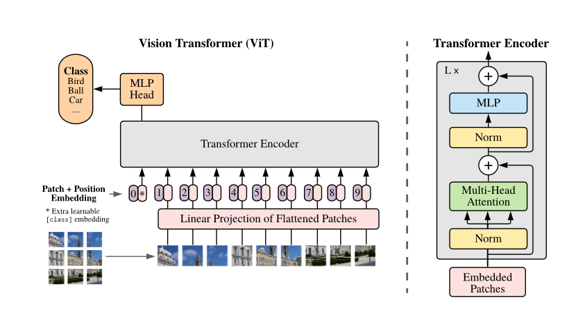
可以看到，ViT的架构与bert几乎完全一样，只不过bert的输入是word embedding + positional embedding，ViT的输入是patch的linear projection + position embedding。不过需要指出的是，ViT是有监督的。 ViT的训练步骤如下：

patch embedding：输入224x224，patch大小16x16，则输入序列长度为196，每个patch维度为16x16x3=768。经过768x768的linear projection之后维度为196x768。由于在前面需要加一个特殊字符[cls]，因此最终的维度是197x768。
positional encoding：与patch embedding相加得到最终结果，有以下三种：
- 1-D pos emb：只考虑patch flatten之后的相对位置信息
- 2-D pos emb：同时考虑X轴和y轴的信息
- rel pos emb：
MHA

关于位置编码

不管使用哪种位置编码方式，模型的精度都很接近，甚至不适用位置编码，模型的性能损失也没有特别大。原因可能是ViT是作用在image patch上的，而不是image pixel，对网络来说这些patch之间的相对位置信息很容易理解。

混合模型

在数据量较小时，混合模型比较占优，但较大时会被Transformer超越。

图像分类方法

在原论文中，为了执行分类任务，作者在编码时引入了NLP界常用的[cls]标签，但也可以使用传统的average pooling，两种方法较为相近。

数据集

ViT只在较大数据集上占据优势。

code

MLP

ViT中的MLP和Transformer中的没有太大的区别：

1
2
3
4
5
6
7


MLPBlock(
  (0): Linear(in_features=768, out_features=3072, bias=True)
  (1): GELU(approximate=none)
  (2): Dropout(p=0.0, inplace=False)
  (3): Linear(in_features=3072, out_features=768, bias=True)
  (4): Dropout(p=0.0, inplace=False)
)

当然，注意到代码中对MLP层进行了初始化：

 1
 2
 3
 4
 5
 6
 7
 8
 9
10


class MLPBlock(MLP):
    """Transformer MLP block."""
    def __init__(self, in_dim: int, mlp_dim: int, dropout: float):
        super().__init__(in_dim, [mlp_dim, in_dim], activation_layer=nn.GELU, inplace=None, dropout=dropout)

        for m in self.modules():
            if isinstance(m, nn.Linear):
                nn.init.xavier_uniform_(m.weight)
                if m.bias is not None:
                    nn.init.normal_(m.bias, std=1e-6)

Encoder Layer

基本结构如下：

 1
 2
 3
 4
 5
 6
 7
 8
 9
10
11
12
13
14
15


EncoderBlock(
  (ln_1): LayerNorm((768,), eps=1e-06, elementwise_affine=True)
  (self_attention): MultiheadAttention(
    (out_proj): NonDynamicallyQuantizableLinear(in_features=768, out_features=768, bias=True)
  )
  (dropout): Dropout(p=0.0, inplace=False)
  (ln_2): LayerNorm((768,), eps=1e-06, elementwise_affine=True)
  (mlp): MLPBlock(
    (0): Linear(in_features=768, out_features=3072, bias=True)
    (1): GELU(approximate=none)
    (2): Dropout(p=0.0, inplace=False)
    (3): Linear(in_features=3072, out_features=768, bias=True)
    (4): Dropout(p=0.0, inplace=False)
  )
)

结构同样模仿transformer，此处不再赘述。

 1
 2
 3
 4
 5
 6
 7
 8
 9
10


def forward(self, input: torch.Tensor):
    torch._assert(input.dim() == 3, f"Expected (batch_size, seq_length, hidden_dim) got {input.shape}")
    x = self.ln_1(input)
    x, _ = self.self_attention(query=x, key=x, value=x, need_weights=False)
    x = self.dropout(x)
    x = x + input

    y = self.ln_2(x)
    y = self.mlp(y)
    return x + y

Encoder

Encoder在堆叠EncoderLayer的基础上，引入了最后一层的norm和embedding：

1
2
3
4


def forward(self, input: torch.Tensor):
    torch._assert(input.dim() == 3, f"Expected (batch_size, seq_length, hidden_dim) got {input.shape}")
    input = input + self.pos_embedding
    return self.ln(self.layers(self.dropout(input)))

这里要注意一下embedding。原文中尝试了3种embedding，但结果类似。此处看上去使用的是1d-embedding，形状为[1, 197, 768]。

Vision Transformer

 1
 2
 3
 4
 5
 6
 7
 8
 9
10
11
12
13
14
15
16
17
18


def forward(self, x: torch.Tensor):
    # Reshape and permute the input tensor
    # [2, 3, 224, 224]
    x = self._process_input(x) # [2, 196, 768]
    n = x.shape[0]

    # Expand the class token to the full batch
    batch_class_token = self.class_token.expand(n, -1, -1)
    x = torch.cat([batch_class_token, x], dim=1) # [2, 197, 768]

    x = self.encoder(x) # [2, 197, 768]

    # Classifier "token" as used by standard language architectures
    x = x[:, 0] # [2, 768]

    x = self.heads(x) # [2, 1000]

    return x

首先重点关注图像的预处理部分self._process_input(x)：

 1
 2
 3
 4
 5
 6
 7
 8
 9
10
11
12
13
14
15
16
17
18
19


def _process_input(self, x: torch.Tensor) -> torch.Tensor:
    # [2, 3, 224, 224]
    n, c, h, w = x.shape
    p = self.patch_size
    n_h = h // p
    n_w = w // p

    # (n, c, h, w) -> (n, hidden_dim, n_h, n_w)
    x = self.conv_proj(x) # [2, 768, 14, 14]
    # (n, hidden_dim, n_h, n_w) -> (n, hidden_dim, (n_h * n_w))
    x = x.reshape(n, self.hidden_dim, n_h * n_w) # [2, 768, 196]

    # (n, hidden_dim, (n_h * n_w)) -> (n, (n_h * n_w), hidden_dim)
    # The self attention layer expects inputs in the format (N, S, E)
    # where S is the source sequence length, N is the batch size, E is the
    # embedding dimension
    x = x.permute(0, 2, 1) # [2, 196, 768]

    return x

224x224的图像，16x16的patch，所以一共有196个patch。可以把它们看成一个“句子”，之后送入transformer，就和NLP、Speech里做得一样了。这里特别注意一下self.conv_proj(x)：

1
2
3


self.conv_proj = nn.Conv2d(
    in_channels=3, out_channels=hidden_dim, kernel_size=patch_size, stride=patch_size
)

注意到这里获取序列的方法是二维卷积而不是线性层。

之后，我们将可学习参数self.class_token拼接到序列之前，投影时将分类token取出来即可用于分类。

1

self.class_token = nn.Parameter(torch.zeros(1, 1, hidden_dim)) # torch.Size([2, 1, 768])

使用总结：

1
2
3
4


img = torch.randn((2, 3, 224, 224))
vitimpl = vit_b_16()
output = vitimpl(img)
print(output.shape)